Tutorials#

Basic collRC functionality#

Calculating reaction coordinates#

Rendering a system#

Animating simulations#

Once you’ve made a style using one of the built-in color schemes, rendering and animating a trajectory is a straightforward as calling animate:

import gsd.hoomd

from coloring import ColorBase
from render import render_npole, animate

style = ColorBase(dark=True)
figure_maker = lambda snap: render_npole(snap, style=style, PEL='contour', dark=True, figsize=5, dpi=500)

fps = 10
with  gsd.hoomd.open('./qpole1.gsd', 'r') as traj:
   # here you might index the trajectory to select fewer frames, i.e. traj[::10].
   print(f'Animating trajectory with {len(traj)} frames will have duration {len(traj)/fps} seconds at {fps} fps.')
   animate(traj, figure_maker=figure_maker, outpath='./base-qpole1.mp4', fps=fps)

Practical examples#

Rectangles in a coplanar electrode#

The following code demonstrates how to use the defect-driven color schemes to render movies which highlight defects in systems of self-assembling rectangles. Both ColorS2Defects and ColorC4Defects have functionality which lets us set a background color scheme for the nondefective particles (ColorEta0 and ColorConn respectively).

Below we’ve included the movies for rect2.gsd in the tutorials/ folder on the github repository, rendered using both color schemes.

Discs on a spherical surface#

We can use ColorC6Defects to highlight defects in crystalline domains on curved surfaces.

Correctly comparing bond orientational order on curved surfaces requires using the gradient of the implicit function to compute local tangent planes and the rotations between them. Without providing this function (left), we see many artificial c6 defects whereas including this correction (right) reveals a more coherent defect structure:

Small clusters crystallizing in 3D#

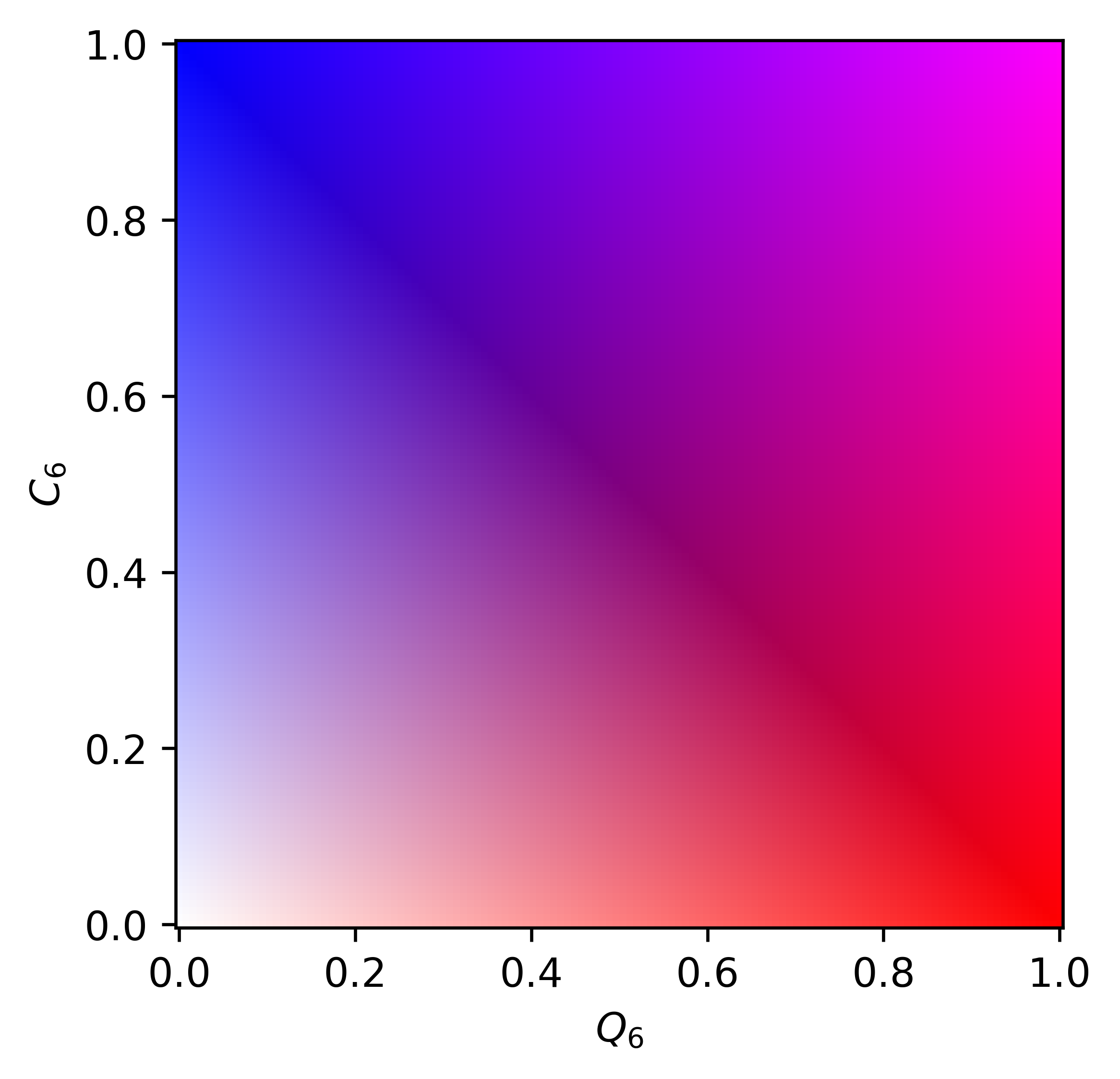
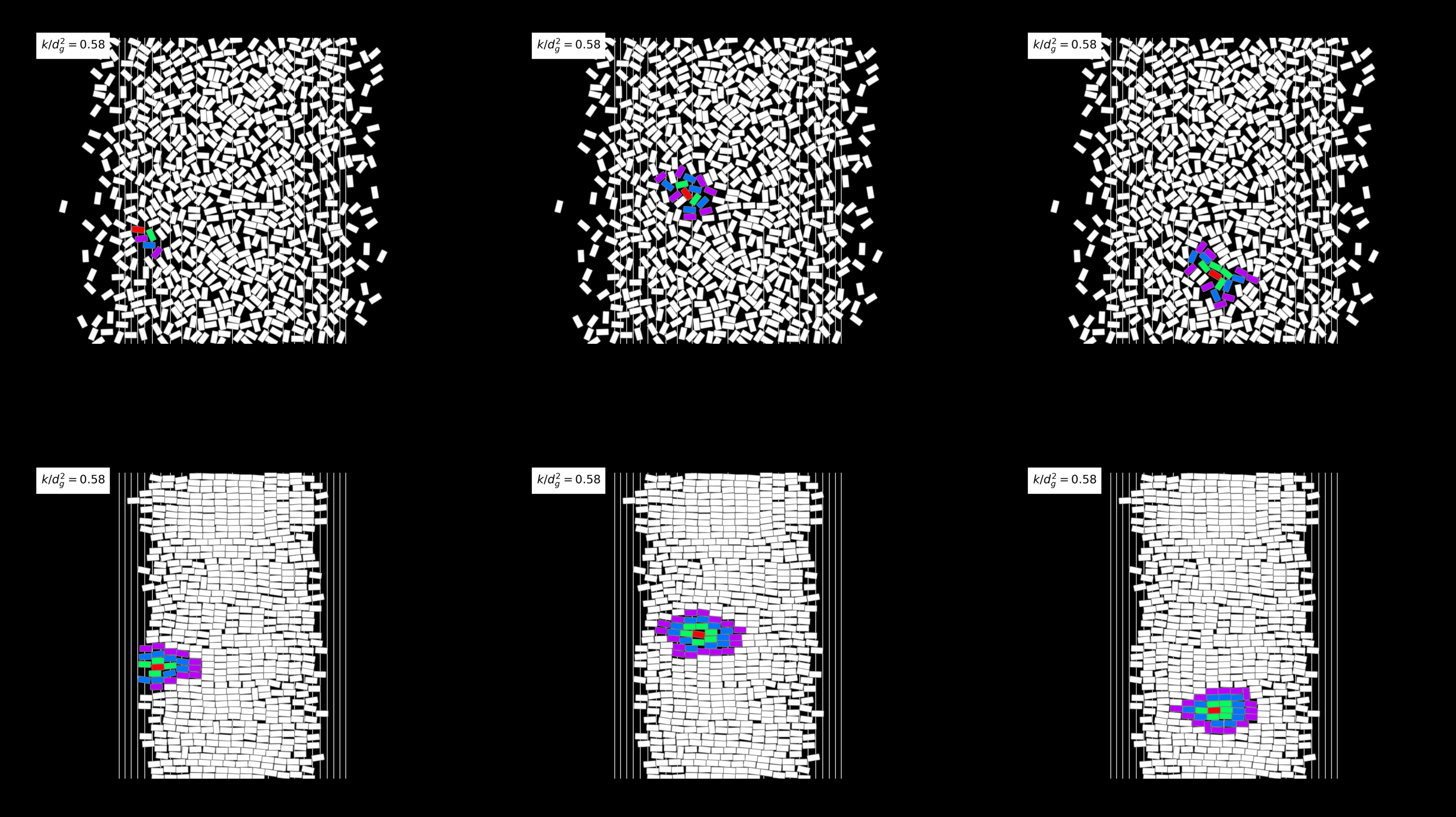
The following code demonstrates how to blend two defect-driven color schemes, using ColorBlender, to show the emergence of local, then global, bond orientational order in small clusters which crystallize at a specific osmotic pressure of deplentants. By instantiating a ColorQG style and a ColorConn style, we can blend them together with a custom colormap to render both at once.

Which produces this movie (and accompanying colormap):

Custom reaction coordinate renders#

Inheriting ColorBase#

You may want to define your own color schemes by inheriting from ColorBase. The basic items to be aware of are the calc_state, local_colors, and color_mapper methods which get called in the render module.

Below we demonstrate how to create a custom color scheme which colors particles based on their nth nearest neighbor distance. We overwrite calc_state (using a @classmethod) to perform the necessary neighbor calculations. We overwrite local_colors to explicitly map those distances to colors using a colormap. In this example we ignore state_string.

At the end of this example we demonstrate a little bit of what goes on in the render module by grabbing the output image from matplotlib as an RBGA array and sticking it on one of several subplot axes:

Inheriting ColorBase subclasses#

collRC already has a lot of reaction coordinates built-in, so often it’s more useful to inherit from an existing subclass of ColorBase so you can focus on adding in your own functionality rather than rewriting existing physics. For example, we can inherit from ColorConn to create a color scheme based on the existing \((\psi_6,C_6)\) fomalism which highlights particles in only in the most prevalent crystalline domains, which helps for exerting control over the morphology and overall crystallinity of a colloidal system.

At the end of the file we demonstrate how to write an extended figure making method, using tools in this module, to animate the principal moments of that most prevalent crystal cluster:

Tutorials

Contents